The analytical framework which allows us to understand these changes and, more importantly, to predict the next ones is rooted in thermodynamics.

Thermodynamic Foundations of Both Supply Side Economics and the Asset Market Shift Framework

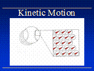
Thermodynamics is the physics of hot coffee cups and cold ice cubes that we live with every day. It is the study of systems of particles. There is no thermodynamics of a single particle. If a group of particles is moving in the same direction—the baseball on the left hand side of Chart 1 on its way from Nolan Ryan’s hand to the catcher’s mitt—we call it coherent energy, kinetic motion, or work. If a group of particles are individually moving in a chaotic manner, jostling against each other but not going anywhere as a group—the baseball in the right hand chart that has been heated in an oven to 350 degrees—we call it incoherent energy, thermal motion, or heat. We refer to the rate at which particles jostle against each other as temperature. The faster they vibrate, the higher the temperature.

Chart 1

1(a): Work 1(b): Heat

Economics studies the interactions of groups of people in markets. Our concerns are work and heat, just like in physics, only we call work “output” and we call heat “cost.”

One of the advantages of this framework is that it gives us a simple way to thing about economic policies. Our objective in engaging in activity is to transform energy into useful work. From this perspective we should measure Gross National Work, not gross national product, which includes the market value of the heat we generate, such as transactions costs and litigation expenses.

Excessive tax rates, subsidies to inefficient producers, and trade restrictions are examples of bad policies; they create heat and destroy work. Policies that increase work are good policies.

From this perspective, the proper target for monetary policy is zero real asset inflation, i.e., zero capital gains for the existing stock of tangible assets. This would focus investors’ attention on the underlying cash flows of an investment, and force wealth creating energies into the security markets where they can finance new capital formation. To a first approximation, this means following a price rule with stable land, property, and commodity price values.

Economics, like physics, is a statistical science; our predictions only hold on average. We rely on the Central Limit Theorem, which says the average of a large number of strange things behaves in a normal, and more or less predictable, way. The spirit of Heisenberg’s Uncertainty Principle holds for economics just as it does for physics. Although we analyze the forces that affect individuals in microeconomics, we have no more ability to predict the behavior of one individual than a physicist does of predicting the behavior of one particle. That’s why command economies where a single individual exerts unusual influence over an economy—dictators, demagogues, and central planning—often degenerate into chaos.

The laws of thermodynamics state, among other things, that a temperature differential cannot persist between two objects that are in contact, or thermal communication, with each other. Their temperatures will tend to move together until they reach the point of thermal equilibrium at which the temperatures are equal. After that, the interesting part is over; nothing further happens.

Thermal equilibrium is the physicist’s definition of death. Anyone who has ever put hot French fries and a cold can of Coca Cola in the same lunch bag learned this lesson the hard way.

Physicists refer to a temperature differential as an energy source. They are the primary engines of change in all physical processes. The process of heat dispersion makes things happen.

Everyone knows one example of this, the storm fronts you see on the weather map. The temperature and atmospheric pressure differentials that constitute weather systems lead to thunderstorms, tornadoes, and hurricanes. Similar forces cause volcanic eruptions, earthquakes, and even chemical reactions. All are examples of cooling activity.

Chart 2

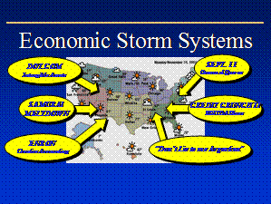
In the same way, we can track return differentials in economics as a set of storm systems that sweep across the economy, as shown in Chart 2.
In economics, we call this phenomenon arbitrage. A price differential cannot persist between two identical goods or services where buyers and sellers are in contact. In fact, we use this condition to define the term “market,” a domain within which prices tend toward equality. People buy low and sell high, driving low prices up and high prices down until they are equal. They release vast amounts of energy as they do.

Arbitrage is what we all do every day in living our lives. We arbitrage gasoline prices between local gas stations. We arbitrage prices of bottles of shampoo at the grocery store. We arbitrage waiting times when we choose which line to stand in at the checkout counter. We arbitrage labor decisions, savings decisions, investment decisions, and trade decisions, whether across town or across the world.

There is only one positive statement in all of economics. “People arbitrage relative price differentials.” The statement that people make choices to improve their wealth is the essence of supply side economics. Just like thermodynamics, the power of supply-side analysis derives from its simplicity and its universal applicability.

If an analysis cannot be reduced to a description of people engaging in arbitrage activities it is simply not economics. Unfortunately, as it is usually taught and practiced, macroeconomics fails this test.

What’s Wrong With Macroeconomics

In macroeconomics students learn that the government can control the economy by manipulating spending and tax rates. They learn about the Phillips Curve, a rhetorical smokescreen for politically-driven tax, spending, and regulatory policies, which leads to the nonsensical conclusion that the act of people working creates inflation. They learn that interest rates are determined by the Federal Reserve, by budget deficits, and by flows of funds. Worst of all, they learn that our wealth and standard of living are determined by how much money we spend—the misleading Y=C+I+G found in all the textbooks—not by how hard we work, what we create, or how much we save and invest.

Students should be learning what arbitrage looks like writ large when it is conducted by large numbers of people in the asset markets. This requires an understanding of balance sheets.

The Island Economy

Macroeconomics textbooks begin by describing how to define and measure economic activity on a hypothetical island economy of Chart 3. Some people on the island catch fish, others pick coconuts. They exchange fish and coconuts with each other (presumably so they get all two major food groups). The island economy’s GDP is measured by adding together the fish and coconuts produced in a year, using the market exchange rate. Although, in practice, GDP is invariably measured by adding up people’s spending over a year, it is intended to be a measure of productive work, much as we would measure the output of a business with a profit and loss statement. Since both fish and coconuts are perishable–you catch it, you eat it—GDP also equals total consumption for the year. Saving and investment both equal zero.

Chart 3
The Textbook Island Economy

There are also no capital markets—no assets—in the island economy. The perishable nature of both fish and coconuts mean it is not possible to produce in one period and consume in the next.

Some writers, such as the great French economist Maurice Allais, have introduced an asset by allowing people on the island to write handshake IOU’s, effectively saying “If you allow me to eat some of the fish and coconuts that you produce this year I will promise to allow you to eat some of the fish and coconuts I produce next year.” With single asset metaphor—the IOU—Allais showed that some demographic patterns can result in a negative equilibrium real interest rate. As I will show below, however, the interesting questions of capital markets only arise when there are many assets, when real goods are storable, and when people are able to make choices among alternative ways to store wealth.

Don’t Forget the Volcano!

I actually live on the island of Maui, so I know something about island economies. There fish in the ocean in front of my house and coconuts in the back yard, just like in the textbooks. When I go to sleep every night, however, I don’t worry about the fish or the coconuts. I worry about the volcano the island is sitting on. If the volcano erupts during the night, tomorrow is going to be a very bad day.

The $10 trillion US economy sits on top of a volcano too, our $100 trillion balance sheet. Even small disturbances in such a huge base of assets can make waves so large that they swamp the effects of the changes in spending, savings rates, budget deficits, and other “flow” measures—the fish and the coconuts—that macroeconomics talks about. These tidal waves of change are transmitted to people’s lives through changes in asset prices.

The Asset Market Shift Framework

In the late 1970’s, Jimmy Carter was President. Inflation, tax rates, government spending, and interest rates were all rising, growth was stagnant, and the dollar was dropping like a brick. Real estate and commodities were soaring. The stock and bond markets were a mess.

Accepted wisdom was that inflation did not matter much for the real economy. After all, labor and product contracts could be indexed and interest rates would rise by just enough to compensate savers for their expected loss of purchasing power—a view mistakenly attributed to the great economist Irving Fisher—leaving real interest rates unchanged.

Irving Fisher, like Knut Wicksell, John Maynard Keynes, and Boehm-Bawerk, understood the lessons of the periodic deflations and financial panics that had plagued western countries between the Civil War and the 1930’s. Monetary, credit, and tax disturbances have major effects on both real interest rates and real economic activity.

Accepted wisdom was not doing a very good job explaining the 1970’s. About that time I found an extraordinary set of data that reported the market value of people’s holdings of tangible assets, such as land, houses, capital goods, consumer durables, and commodities. They were huge, bigger than any numbers macroeconomists were writing about.

What intrigued me most was that macroeconomics had no analytical pigeon hole for this data. According to James Tobin, in flowchart contained in his 1969 Presidential address to the American Economic Association, “the interest rate” was a parameter that was set by the central bank. Asset arbitrage, which his students later had the hubris to call “Modern Portfolio Theory,” was confined to security markets. Interest rates influenced the real production economy through their effects on investment decisions, but the real economy did not in turn influence interest rates. Real assets did not exist.

How could that be, I wondered. Interest rates were simply prices of a particular subset of people’s assets. People owned real assets too. The largest asset class was real estate, not securities. Didn’t this leave out the star of the play?

This seemed to me like the joke going around about the US government’s refusal to recognize the one billion people in China. How could we not recognize the largest asset class in the country?

My colleagues and I built the asset market shift framework to give Hamlet back his speaking part in the play. We used it to great effect during the latter stages of the Carter inflation to predict the effects of rising inflation and tax rates on interest rates and commodity markets. This framework unified the behavior of the hard asset markets with the security markets and explained why variations in inflation and tax rates exert powerful real effects on interest rates, asset values, and real wealth accumulation. It rests entirely on arbitrage behavior.

In November 1981, I wrote a piece describing this framework for the Wall Street Journal's Op-Ed page. The article was called "Why Interest Rates Must Fall in 1982". At that time, Wall Street economists were divided between those who, like Dr. Doom and Mister Gloom, believed Reagan’s tax cuts would lead to big budget deficits, and rising interest rates, and those who argued that Reagan’s tax cuts would stimulate more savings and drive interest rates down.

I argued that the course of interest rates would not turn on savings or deficits. Instead, the Reagan Administration’s economic plan contained inflation and tax rate reductions that were going to turn the asset markets on their head by forcing massive private sector asset arbitrage. These asset arbitrage activities would lead to a reversal of all the major trends of the 1970’s. Interest rates had to fall, regardless of the budget deficit. Deficits and savings rates would be rounding errors in the biggest portfolio event of the century.

I didn’t get many dinner invitations from fellow economists after that. But I did make a lot of money. Here are the bones of the framework that made this possible.

As economists, we have two price theories in our tool box. The first—supply and demand—is the price theory of Alfred Marshall and George Stigler. It works well for haircuts, guitar lessons, and other perishable goods and services. The second—portfolio theory—is the price theory of Irving Fisher, Knut Wicksell, John Maynard Keynes, Milton Friedman, and James Tobin. It works for bonds, Rembrandt paintings, the stock of money, and other storable assets. To get the right answers we have to use the right tool.

Alfred Marshall’s price theory is for goods and services that have a large rate of current production relative and small existing stockpiles. It works for perishable items like masseuse services (it’s over before you know it), airline seat miles, and fresh strawberries (they rot in one day).

Irving Fisher’s price theory is for assets that have large stockpiles and low rates of production. It works for durable goods like Rembrandt paintings (he is not painting any more), ’57 Chevy’s (the best car ever made, pronounced with a hard ch, as in Cheech and Chong,) and beachfront property (they aren’t making any more.)
We can measure the “asset-ness” of different products with a parameter I will call alpha which I will calculate by dividing the existing stockpile by a year’s production. Alpha gives us a pretty good sense of where each product fits in the stock/flow continuum.
Most products are somewhat storable but wear out over time. They have alphas larger than haircuts and smaller than Rembrandts. Medical services, food, and apparel are all pretty much goods and services—their alphas will all be close to zero. Land, homes, copper, gold, and even automobiles (there are 150 million used cars, about 10 years production) will have alphas between 15 (for cars) and infinity (for land). They behave like assets.

Bonds are assets. On March 31, 2002 the total existing stockpile of government debt—the national debt—was $6.01 trillion. Of that total, $3.39 trillion was held by the public and the rest owned by government agencies. This year, the federal budget deficit will be about $130, i.e., the federal government will produce and sell $130 billion of new debt. Using these numbers we can calculate the alpha for government debt as either 46.2 or 26.2 depending on which definition of government debt you prefer to use in the numerator. Either way, the outstanding stock of bonds is many years’ new supply.

That means the supply of bonds will be almost invariant to price, i.e., we can view the supply curve as vertical. In this situation, bond prices, and therefore interest rates, on any given day will be insensitive to government financing activities. Interest rates are entirely determined by demand—whatever they need to be to make people willingly hold the existing stock of bonds. The mechanism that makes this work is portfolio balance, the asset market analog of arbitrage and thermodynamic adjustment at the micro level.

Asset Market Equilibrium

This seems like a good time to drop in some paragraphs of facts about the balance sheet of the US economy. Problem is there aren’t any—at least not for the whole economy. So we will h ave to piece it together from the building blocks we can find.

I know you are wondering how this sorry state of affairs came to be in a country where you can’t walk across the street without tripping over a time series. Between the efforts of the Commerce Dept., the Bureau of Labor Statistics, the Treasury Dept., the Federal Reserve, the International Energy Agency, the IMK, the World Bank, and the OECD, I can tell you how many left-handed Armenians played squash in the third week of April. But I can’t tell you how much stuff we owned at the end of last year.

The Flow of Funds Division of the Federal Reserve Board used to publish a biannual report called “Balance Sheets of the United States,” which contained a consolidated balance sheet for the country along with separate balance sheets for all the sub sectors along with a full set of annual data since 1948.

The Fed stopped publishing the report in 1995. This is understandable from a cost-benefit point of view since the report was read by only one person—me. Frankly, I am hoping this article will stimulate a tsunami of interest in the subject. If we can get three of four of us together we might get the Fed to bring the report back to life.

The real reason it was dropped, of course, is there is no place for non-financial assets in the standard Keynesian model that dominates thinking both at the Federal Reserve Board and in the economics profession.

When I first discovered the data set 25 years ago I was struck by two facts. 1) Tangible asset holdings, especially real estate, are huge—the biggest numbers on the page. 2) The net worth of the US economy is always almost exactly equal to the market value of our tangible asset holdings. A little reflection convinced me this must be true.

If you start in a jungle book world of hunter-gatherers there are no financial assets or liabilities—stuff is all there is. In that world total assets equal the value of tangible assets, total liabilities equal zero, and net worth is exactly equal to tangible wealth.

As we depart from that simple world we create financial assets and liabilities but net worth remains equal to the market value of tangible wealth. This is obvious for the debt markets where one man’s claim is another man’s IOU. It is also true for the equity markets where the duality between a competitive market for valuing productive assets and a competitive financial capital market—the stock market—for valuing streams of future free cash flows produced by those assets ensures that the value of future product is reflected in the current market value of tangible assets. This is the root of the capital problem, the legendary under identification problem that has plagued capital theorists for centuries.

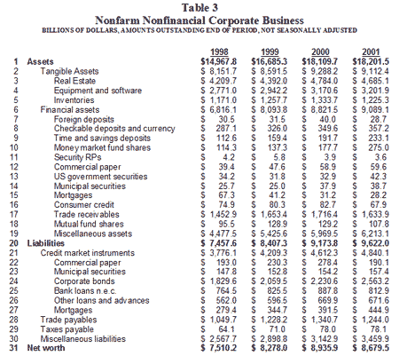
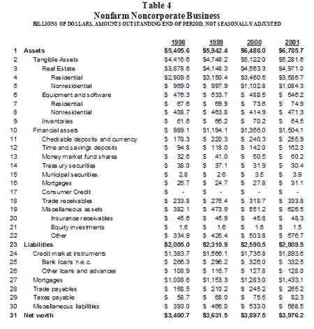
The Fed does, however, deign to publish balance sheets for three sectors: 1) households and nonprofit organizations, 2) nonfarm, nonfinancial corporate business, and 3) nonfarm, noncorporate business as an addendum to their regular quarterly flow of funds accounts. Each can be analyzed to understand the portfolio decisions of the market participants in that sector. I have included the most recent data for all three sectors at the end of this article.

In principle we can add the sectors together to produce a consolidated balance sheet—the work the Fed once did for us. In practice, however, it is not a simple exercise since the data are not reported in a form that the necessary inter-sectoral eliminations easy to do. A simple aggregation, however, in which we do not attempt to do a proper consolidation gives a valuable illustration of the size and composition of the asset markets.

The table below shows the result of adding together the three sectors reported by the Federal Reserve Board.

The first thing you notice about the balance sheet is its sheer size. This should not come as a shock. Total assets represent the cumulative sum of all human effort since Adam and Eve, plus our endowments of natural resources. It would be a shock if this number were small.

Total assets (line 1) at the end of last year were $72.9 trillion, equal to 9.8 times (line 11) our annual disposable income (line 10). Tangible assets makes up $30.7 trillion (42%) of that total, including $22.9 trillion in real estate, $3,9 trillion in capital equipment, $2.9 trillion in used cars and washing machines, and $1.3 trillion of inventories. In addition, we own $42.3 trillion (58%) in the form of financial assets.

On the other side of the ledger we have a $20.5 trillion of liabilities, which equals 28.1% of total assets and 38.9% of our net worth. Our net worth is 5.38 times our disposable income. Americans are not as highly leveraged as the pessimists would have us believe.

Remember, these data only measure part of the economy. We have left out financial institutions—all those tall bank buildings—and foreign holders of US assets. More important, we have (mostly) left out the government. We did include government securities in the sector assets, which added $1.2 trillion to net worth. We did not, however, include either government liabilities or government tangible asset holdings. Federal government debt held by the private sector is $3.4 trillion, state debt another $__ trillion. Those numbers are easy to get. Not so easy to get, however, are data on government real asset holdings.

The GAO once issued a balance sheet for the federal government in which they listed, among other assets, more than 750 million acres of land owned by the government. They valued the land at $1 per acre to construct the balance sheet, which allowed then to show a government sorely in debt. If we were to place any reasonable valuation on the land and other tangible assets owned by the government the federal government would show a sizeable net worth and the net worth numbers reported above in Table 1 would rise still higher. I will save the government balance sheet for another time.

Chart 4
The US Household Balance Sheet; December 31, 2001

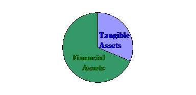
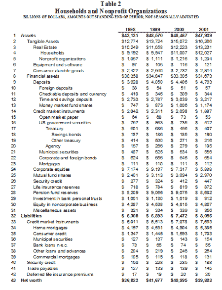
Households and nonprofit organizations owned $47.9 trillion of total assets on December 31 2001, shown in Chart 4. Of these, $16.3 trillion, or 33.9%, were held as tangible assets. The remaining $31.7 trillion, or 66.1%, were held as financial assets, like bonds, stocks, and money market funds. This $47.9 trillion in assets was partially offset by total liabilities of $8.1 trillion. Debt 16.8% of total assets is not much leverage—in spite of what you read. Net worth was a whopping $39.9 trillion.

Chart 5

Portfolio balance, or asset market equilibrium, refers to the situation of thermodynamic equilibrium depicted in Chart 5 in which returns on tangible and financial assets are just equal so that owners are content to hold the existing stock of assets. In portfolio equilibrium there are no arbitrage opportunities for investors to exploit -- asset prices remain at current levels.

Asset Market Arbitrage Makes Things Happen

Anything that materially alters the relative risks or returns of the assets in the portfolio tilts the scale in Chart 5. This leads investors to select a preferred asset mix different from the one they own. They then attempt to change their portfolio by buying or selling assets in the market. In the aggregate, this forces asset prices to change until investors are again content to own the existing assets.

I have split the US balance sheet into tangible and financial assets because inflation and tax rates affect the returns of these two categories so differently. Inflation is a direct component of the total return on tangible assets but not for financial assets. Increased inflation will cause households to attempt to shift their portfolios toward tangible assets, and away from financial assets. As a group, however, they cannot accomplish this. Their efforts to do so, however, will drive tangible asset prices up and financial asset prices down, i.e., interest rates up, until the composition of the revalued assets matches asset demands and portfolio balance is again restored.

Likewise, an increase in tax rates will reduce the after-tax return of financial assets relative to tangible assets (since the yield on tangible assets is generally non-taxable). This will shift relative asset demand toward tangible assets, which will drive their prices up and financial asset prices down, until portfolio balance is once again restored.

This is what Irving Fisher wrote about more than 100 years ago when he examined the link between inflation and interest rates. Inflation and tax rates influence interest rates and asset prices through their effects on relative after-tax returns on tangible and financial assets—real interest rates. Chapter 17 of Keynes’s General Theory is the most cogent description of these issues ever written.

Real interest rates should be measured using tangible asset inflation, not CPI inflation, to ensure that the result reflects the after-tax return spread between tangible and financial asset yields that drives investor behavior. Measured properly, this tangible real rate is the economic analog to the temperature differential that serves as the fundamental energy source in thermodynamics.

Chart 6

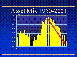
During the past twenty years, as Chart 6 shows, households have systematically reduced tangible asset holdings as a percentage of total assets from 43% in 1981 to 32% today. This has pushed interest rates to their lowest rates in forty years and pushed stock price multiples to historic highs. It has also played havoc with the economics of durable goods industries that are forced to compete with mountains of their own previously produced products selling at discounted prices in the secondary markets.

Chart 7
Relative Price of Financial Assets to Tangible Assets
S&P 500 INDEX DIVIDED BY MEDIAN PRICE OF AN EXISTING HOME

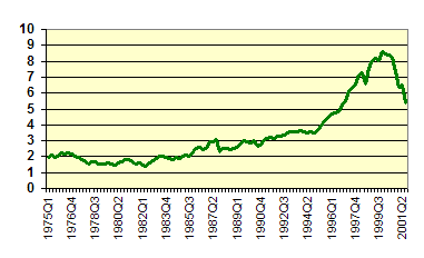
Chart 7 shows the S&P 500 index as a multiple of the median price of an existing home. Stocks were valued at two median homes during most of the 1980’s. Stock prices increased to four homes in 1996, and peaked at more than eight homes during the dot-com boom in late 1999 before falling to about six homes today.

Chart 8

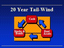
During this twenty year run, as a result of the asset price pressures shown in Chart 8, home builders, commodity producers, and durable goods manufacturers faced a powerful headwind, with continual fixed-asset write-offs and margin pressure from weak resale markets. Owners and producers of financial assets, in contrast, such as stock market investors, brokerage firms, and mutual funds, enjoyed a strong tailwind. For them, it was easier to make profits.

Schools, guidance counselors, and graduating students followed the path of least resistance. We went from being a nation of real estate brokers to a nation of stockbrokers.

Whether the reversal of the twenty year trend over the past two years we saw in Chart 8 will continue is the most important question for investors today. As we saw in Table 1, tangible assets have already risen from their trough of 24.7% of total assets in 1999 to 28.1% of total assets today. Real estate cash returns are very attractive today relative to total return projections for equities.

Ironically, early this year Morgan Stanley provided anecdotal evidence of this shift when they announced they were moving their headquarters to the old Texaco headquarters building they had just purchased in Rye, New York. That serves as a pretty good indicator that the balance sheet event I have been describing has gone on too long.


Balance Sheets Today: A Gleaner’s Market

Asset market disturbances are one-trick ponies, even big ones like I have been describing. Like hurricanes, when they are over, they are over. For good or ill, this one is over now. Balance sheets have now fully adjusted to today’s inflation and tax rates. This leaves us with two things to do, clean up the mess left by the storm, and start watching out for the next one.

We have a fair amount of mess to clean up. Most of it takes the form of squeezing the hubris out of the people who got the erroneous impression that it was their efforts, rather than the tidal wave of price change, that made them rich. Day traders and momentum investors are one cohort of this group. The managers of ENRON, TYCO, Global Crossing, Vivendi, and others who found accounting rules too confining, along with their domesticated watchdog auditors, are another. The dot.com binge, venture capital investors, pension fund managers, and conflicted analysts and investment bankers are a third.

Unfortunately, the clean up will also spawn witch hunts, like the ones now taking place on C-Span every day.

The final mess we have to clean up is inside our heads. We all have to learn that the incredible Reagan Run of the last twenty years is over now. From now on we are going to have to actually earn the money.

Bummer.

For two decades, the biggest mistake an investor could make was to be out of the market. We made our money by betting on rising valuations, not rising performance. Momentum investing worked, value investing didn’t. Stocks in the S&P index made money, small caps didn’t. An entire generation of investment professionals—four out of every five people now working on Wall Street—was hired fresh out of school and trained during this period—it is all they have ever seen.

The world we are in today is very different. High real growth of 3-4% per year, due to strong productivity gains, and inflation of only 1-2% per year means that GDP growth will only average 4-6% per year. That implies single digit earnings growth and single digit stock market returns. Low interest rates and high multiples mean the new winners will be companies that are able to demonstrate consistently above-average top line growth, systematic cost reductions, and pricing power. Identifying these companies is the work of old-fashioned, bottom-up, value-oriented security analysis. There aren’t many people around today who remember how to do that.

The asset market shifts we experience in the next decade will be different too. Instead of the wholesale repricing of the entire balance sheet, we will be in a gleaner’s market of smaller, shorter-lived, and more geographically dispersed arbitrage opportunities. This is a market where hedge fund investors will have a distinct advantage over larger, slower-moving, long-only investment funds.

These mini-shifts will be like small earthquakes, not important enough to make the 10 o’clock news but big enough to shake things up for the people at the epicenter. They will occur in situations where a localized disturbance to relative returns happens in a spot that is not well covered by the analysts. There are many examples of such opportunities today.

One example is the utility sector—the eye of the witch hunt hurricane. Investors are selling good franchises along with bad ones. Value investors who know the difference will be rewarded handsomely once the witch hunt is over.

A second example is Japan. The economists at the Bank of Japan think they have been stimulating the Japanese economy for more than a decade with budget deficits and low money interest rates. While they have been talking stimulus they have been walking tight money. Land and other real asset prices in Japan have deflating for more than a decade. Tangible real rates have been 10% per year.

Japanese companies—long fixed-assets and short yen debt—have been crushed under the burden of never-ending write-offs, leading to a series of recessions. Their problems cannot be resolved until land prices stop falling. Recently, money growth has exploded and the yen is falling. If this signals a reversal in the decade-long deflation it will be a great opportunity to make money.

A third example is Germany, where capital gains tax rates on cross-shareholdings were reduced to zero earlier this year for public companies. Although political and labor market problems will keep the German economy from growing rapidly, these tax law changes will lead to a substantial amount of restructuring transactions, making merger arbitrage an interesting area for gleaners to exploit.

Fourth, there is pressure in the UK to devalue the pound before joining the EMU. This will undermine the return on some industrial assets and fan the fires of property inflation—already 16.5% last year.

There is no shortage of portfolio disturbances elsewhere. Korea is going gangbusters. Asian economies are recovering. Latin America is morally, politically and economically bankrupt. US trade restrictions on steel and lumber increased flat-rolled steel prices by 30-50% in a month leading to a 50% increase in the market capitalization of specialty producers like Timken. Trade restrictions on lumber have added $1000 to the cost of building a home. Europe, Canada, and Japan are retaliating with restrictions of their own. Oil prices are 40% higher than last year, which has spiked energy sector returns and stock prices. They are unsustainable at today’s levels.

In each of these situations, an event leads to a return differential that, in turn, will attract the attention of arbitrageurs. For those who are able to identify these situations early and put their bets in place, they represent interesting opportunities to earn high returns.